Creating Interaction Categorical and Continuous Variables Spss

1. A standard ANOVA
2. A standard ANCOVA
3. Estimate slopes for each diet group
4. Test equality of slopes across diet groups
5. Perform tests with separate slopes for all diet groups
5.1 Comparing diet 1 with diet 2
     5.2 Comparing diets 1 and 2 to the control group
6. Testing to pool slopes
7. Perform tests with some pooled slopes
  7.1 Overall analysis pooling slopes for diet groups 2 and 3
7.2 Comparing diet groups 1 and 2 when pooling slopes for diet groups 2 and 3
  7.3 Comparing diet groups 2 and 3 when pooling slopes for diet groups 2 and 3
8. Summary

Analysis of covariance (ANCOVA) is a statistical procedure that allows you to include both categorical and continuous variables in a single model. ANCOVA assumes that the regression coefficients are homogeneous (the same) across the categorical variable. Violation of this assumption can lead to incorrect conclusions. This page will explore what happens when you have heterogeneous (different) regressions across groups and show some strategies for dealing with them. This involves some complex topics in the use of the glm command, especially the lmatrix subcommand.

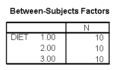
Here is an example data file we will use. It contains 30 subjects who used one of three diets, diet 1 (diet=1), diet 2 (diet=2) and a control group (diet=3). Before the start of the study, the height of the subject was measured, and after the study the weight of the subject was measured.

                data list list / id diet height weight. begin data  1 1  56 140  2 1  60 155  3 1  64 143  4 1  68 161  5 1  72 139  6 1  54 159  7 1  62 138  8 1  65 121  9 1  65 161 10 1  70 145 11 2  56 117 12 2  60 125 13 2  64 133 14 2  68 141 15 2  72 149 16 2  54 109 17 2  62 128 18 2  65 131 19 2  65 131 20 2  70 145 21 3  54 211 22 3  58 223 23 3  62 235 24 3  66 247 25 3  70 259 26 3  52 201 27 3  59 228 28 3  64 245 29 3  65 241 30 3  72 269 end data.              

1. A standard ANOVA

You could analyze this data with a standard ANOVA, as shown below. This analysis compares the weights of the three groups. It uses the /contrast subcommand to compare the two diets (1 and 2) to the control group (diet 3).  We also want to compare diet 1 with diet 2.

                glm weight by diet  /print = descriptive  /contrast(diet) = special(1 1 -2)  /constrast(diet) = special(1 -1 0).              

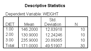
The ANOVA results show an overall difference among all of the diets and the contrasts show a difference between the control group and the two diets, and a difference between diet 1 and diet 2.   The ANOVA disregards the information that we have about the subject's height. As height is probably correlated with weight, this could be useful as a covariate in an ANCOVA.

2. A standard ANCOVA

Below we perform a standard ANCOVA.

                glm weight by diet with height  /emmeans = tables(diet)  /contrast(diet) = special(1 1 -2)  /constrast(diet) = special(1 -1 0)  /print = parameter.              

The results are consistent with those of the ANOVA. There is an overall effect of diet. Also, the control group is significantly different from the two diets, and diet 1 is different from diet 2. The significance level for the comparison of diet 1 versus diet 2 is smaller than the standard ANOVA.

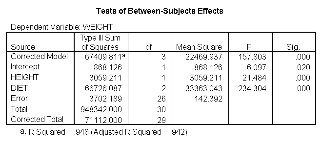
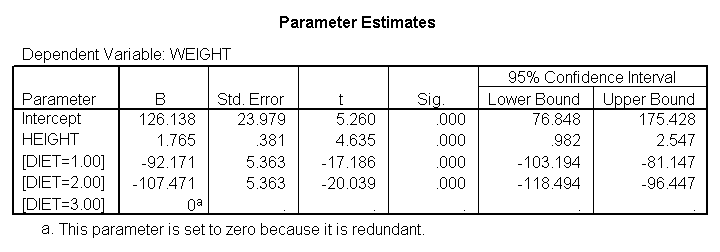
Because we used the print = parameter subcommand, we are shown the regression coefficients and see the coefficient (slope) between height and weight is 1.765. Figure 1 below shows the scatterplot between height and weight and the line of best fit with slope 1.765.

                GGRAPH   /GRAPHDATASET NAME="iGraphDataset" VARIABLES= weight height    /GRAPHSPEC SOURCE=INLINE INLINETEMPLATE=["<addFitLine  type='linear' target='pair'/> "]. BEGIN GPL SOURCE: s=userSource( id( "iGraphDataset" ) ) DATA: weight=col( source(s), name( "weight" ) ) DATA: height=col( source(s), name( "height" ) ) GUIDE: axis( dim( 1 ), label( "height" ) ) GUIDE: axis( dim( 2 ), label( "weight" ) ) ELEMENT: point( position( ( height * weight ) ) ) END GPL.              

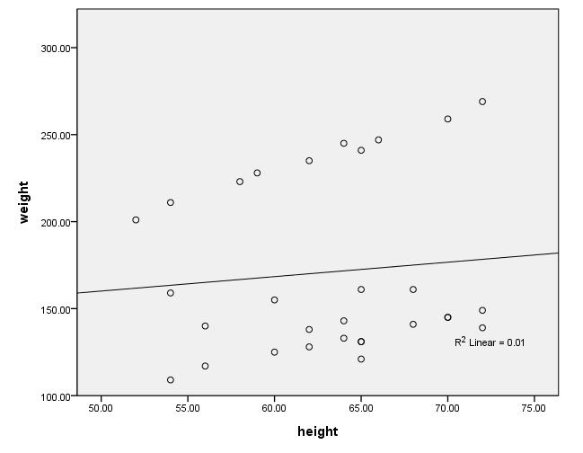
Figure 1. Scatterplot of weight by height with overall regression line

3. Estimate slopes for each diet group

One assumption of ANCOVA is that the slope between height and weight is the same for the three diet groups. This is called the homogeneity of regression assumption. Below we show a scatterplot like the one above; however, this one shows the three diet groups in different colors and shows a separate regression line for each diet group (diet 1=red, diet 2=green, diet 3=blue). As you can see the red regression line looks like it has a very different slope from the other two regression lines.

After running the code below, you will need to double-click on the graph and select "chart" from the menu at the top. Selecting "options" will open up a dialog box. On the right under "fit line" put a check in the "subgroups" box. This will insert the regression lines for each group. You need to use the "by" option (or "set markers by" in the point-and-click interface) in order to be able to add the regression lines for the subgroups. If you do not, when you double-click on the graph to open the chart editor, the "subgroups" option under "Fit Line" will not be available.

                GRAPH /SCATTERPLOT(BIVAR)=height WITH weight BY diet.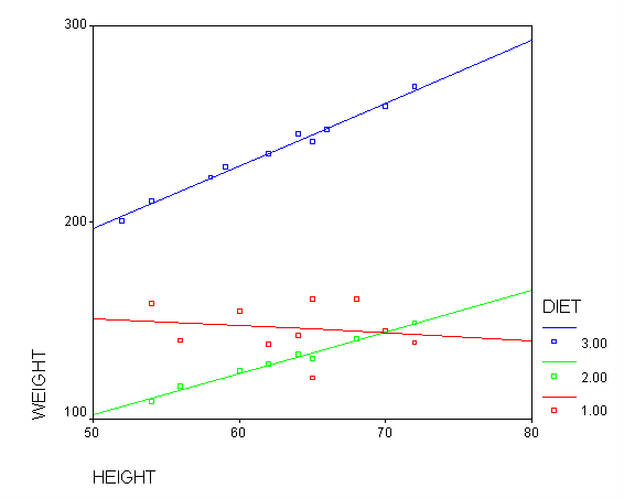              

Figure 2. Scatterplot of weight by height with separate regression lines for each group (diet 1=red, diet 2=green, diet 3=blue)

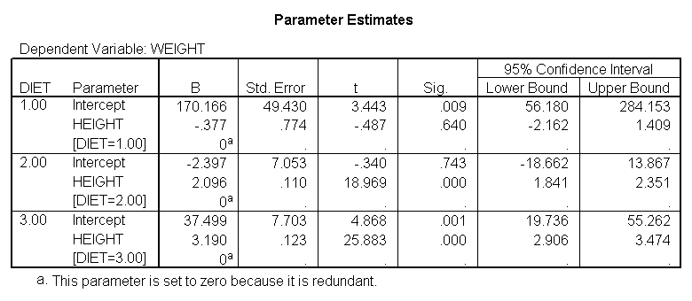
Below we perform an analysis that shows the slopes of each of the lines. Even if we found the slope between height and weight to be 0 in the prior analysis, this is still a useful analysis to perform. It is possible that the overall slope for the entire sample was 0, but the slopes for some groups were positive and the others were negative and they cancelled each other out. This analysis would help you see if such a pattern was occurring.

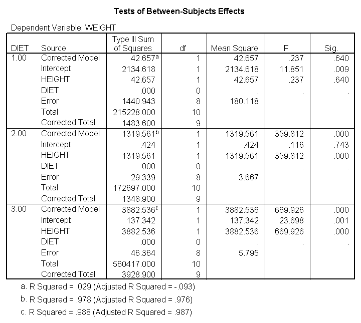
                sort cases by diet. temporary. split file by diet. glm weight by diet with height  /print = parameter.              

We indeed see below that the slopes seem very different. (Note that the output has been abbreviated.)  The slope for diet 1 (-.377) is much smaller than the slope for diet 2 (2.096) and the control group, diet=3 (3.190).  We need to check into this further and test whether these slopes are significantly different from each other.

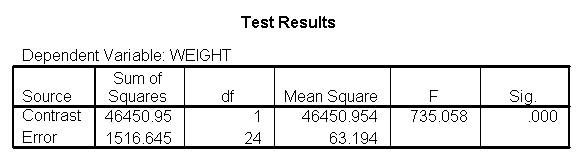
4. Test equality of slopes across diet groups

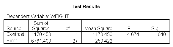
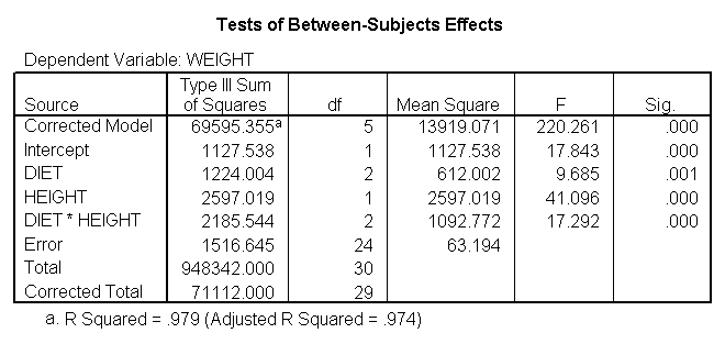
We can test to see if the slopes for the three diet groups are equal, as shown below. The diet*height effect tests if the three slopes are equal.

                glm weight by diet with height  /design diet height diet*height.              

The diet*height effect is indeed significant, indicating that the slopes do differ across the three diet groups. The output is abbreviated to save space.

5. Perform tests with separate slopes for all diet groups

Because the slopes for the three diet groups are not the same, we should not use a traditional ANCOVA model that assumes the slopes for the three diet groups are the same.  Instead, we can use a model that estimates separate slopes for all three diet groups. Because the diet groups will have different slopes, we must be very cautious in interpreting adjusted means. One way of thinking about this is to focus on the fact that we have a diet*height interaction. This means that we cannot interpret the relationship between height and weight without referring to diet. Likewise, if we want to talk about the effect of diet we need to specify what height we are talking about. For example, in comparing diets 1 and 2 (in Figure 2) it looks like there is no difference between diets 1 and 2 (red and green) for tall people, but there may be a difference for shorter people. Below, we will see how to make these comparisons.

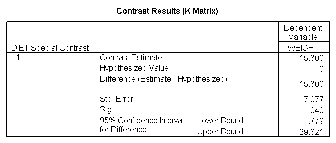
5.1 Comparing diet 1 with diet 2

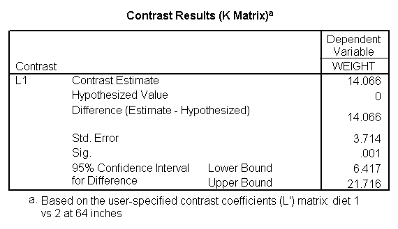
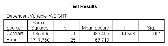
Let us compare diet 1 versus diet 2 at three different levels of height, for those who are 59 inches tall, 64 inches and 68 inches tall. These correspond to the 25th, 50th and 75th percentiles for height. We can then evaluate separately for each height group the difference between diet 1 and diet 2.

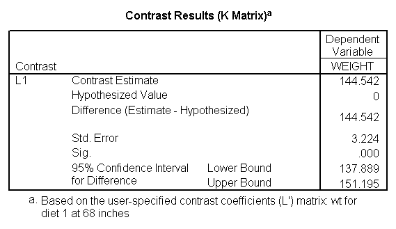
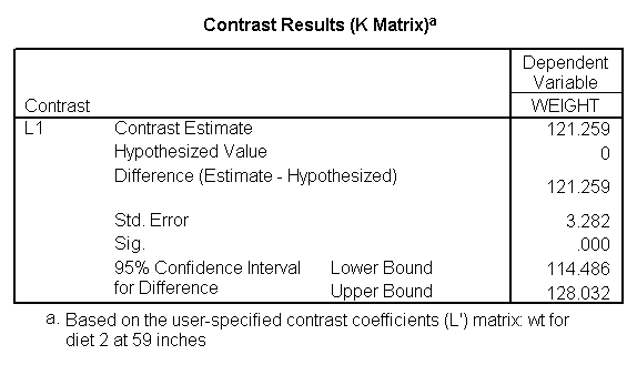
The model used in this analysis is the same as the model from section 4 where we estimated separate slopes. In addition we use the lmatrix subcommand for comparing the diets 1 and 2 at the three levels of height, and for obtaining the adjusted mean for weight.

The first three lmatrix subcommands compare diet 1 with diet 2 at 59, 64, and 68 inches. The next three lmatrix subcommand s request the predicted value of weight for people on diet 1 who are 59 inches, 64 inches, and 68 inches tall. The next three lmatrix subcommand s requests the weight for people on diet 2 who are 59 inches, 64 inches, and 68 inches tall.

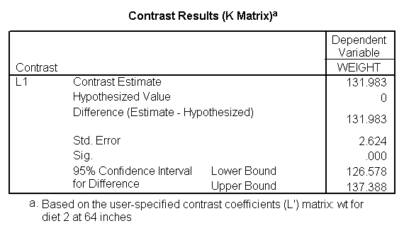
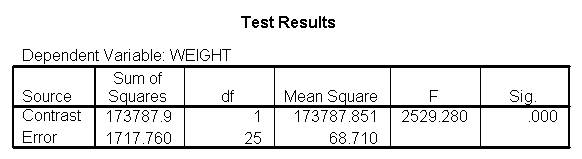
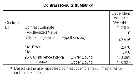
                glm weight by diet with height  /design diet diet*height  /lmatrix "diet 1 vs 2 at 59 inches" diet -1 1 0 diet*height -59 59 0  /lmatrix "diet 1 vs 2 at 64 inches" diet -1 1 0 diet*height -64 64 0  /lmatrix "diet 1 vs 2 at 68 inches" diet -1 1 0 diet*height -68 68 0  /lmatrix "wt for diet 1 at 59 inches" intercept 1 diet 1 0 0 diet*height 59 0 0  /lmatrix "wt for diet 1 at 64 inches" intercept 1 diet 1 0 0 diet*height 64 0 0  /lmatrix "wt for diet 1 at 68 inches" intercept 1 diet 1 0 0 diet*height 68 0 0  /lmatrix "wt for diet 2 at 59 inches" intercept 1 diet 0 1 0 diet*height 0 59 0  /lmatrix "wt for diet 2 at 64 inches" intercept 1 diet 0 1 0 diet*height 0 64 0  /lmatrix "wt for diet 2 at 68 inches" intercept 1 diet 0 1 0 diet*height 0 68 0  /print = parameter.              

For the sake of saving space, we show just the output related to the lmatrix subcommands.

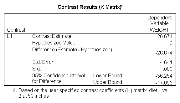
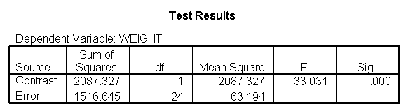
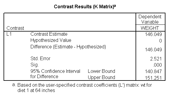
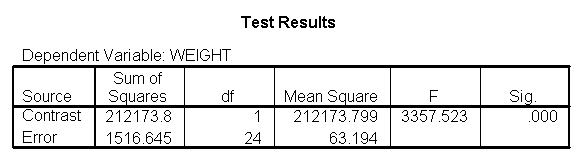
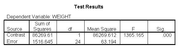
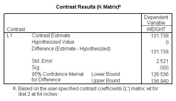
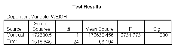
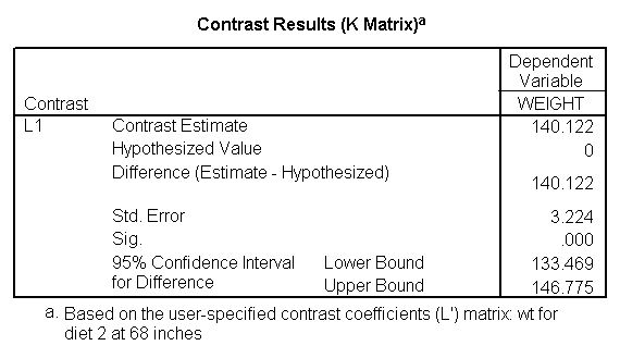
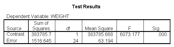
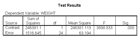
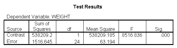
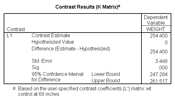
Focusing on the comparison of diets 1 and 2, these results indicate a significant difference between diet 1 and diet 2 for those 59 inches tall (t=-5.75, p < .0001) and a significant difference for those 64 inches tall (t=-4.01, p=0.0005).  For those who are tall (i.e., 68 inches), diet 1 and diet 2 are about equally effective.  This corresponds with what we saw in Figure 2.

You will notice that if you take the parameter estimate for "wt for diet 1 at 59 in" minus the parameter estimate for "wt for diet 2 at 59 in", you get -26.67, which is the parameter estimate for "diet 1 vs. 2 at 59 in" (147.93 – 121.25 = -26.67). Likewise, taking the parameter estimate for "wt for diet 1 at 64 in" minus the parameter estimate for "wt for diet 2 at 64in" yields the parameter estimate for "diet 1 vs. 2 at 64 in" (146.04-131.73 = -14.31).  You can do a similar computation for the weights for those 68 inches tall.

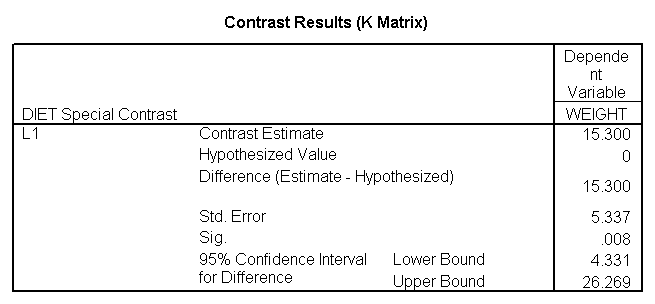
5.2 Comparing diets 1 and 2 to the control group

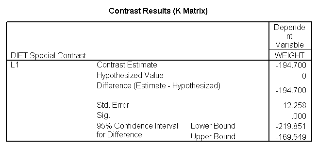
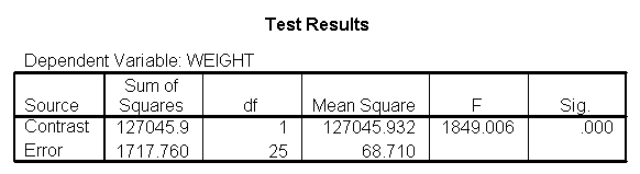
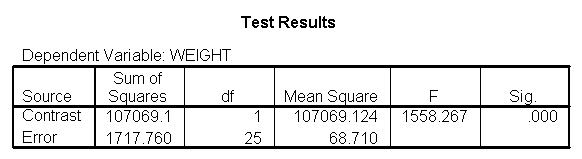
The analysis below compares diets 1 and 2 to the control group (group 3) at the three different heights: 59 inches, 64 inches and 68 inches. The first three lmatrix subcommands compare diets 1 and 2 to the control group at these three different heights. The next three lmatrix subcommands estimate the weight for the diet 1 and diet 2 groups combined at the three heights.  The following lmatrix subcommands estimate the weight for the control group at the three heights.

                glm weight by diet with height  /design diet diet*height  /lmatrix "diet 1&2 vs 3 at 59 inches" diet .5 .5 -1 diet*height 29.5 29.5 -59  /lmatrix "diet 1&2 vs 3 at 64 inches" diet .5 .5 -1 diet*height 32 32 -64  /lmatrix "diet 1&2 vs 3 at 68 inches" diet .5 .5 -1 diet*height 34 34 -68  /lmatrix "wt diet 1&2 at 59 inches" intercept 1 diet .5 .5 0 diet*height 29.5 29.5 0  /lmatrix "wt diet 1&2 at 64 inches" intercept 1 diet .5 .5 0 diet*height 32 32 0  /lmatrix "wt diet 1&2 at 68 inches" intercept 1 diet .5 .5 0 diet*height 34 34 0  /lmatrix "wt control at 59 inches" intercept 1 diet 0 0 1 diet*height 0 0 59  /lmatrix "wt control at 64 inches" intercept 1 diet 0 0 1 diet*height 0 0 64  /lmatrix "wt control at 68 inches" intercept 1 diet 0 0 1 diet*height 0 0 68  /print = parameter.              

For the sake of saving space, we show just the output related to the lmatrix subcommands.

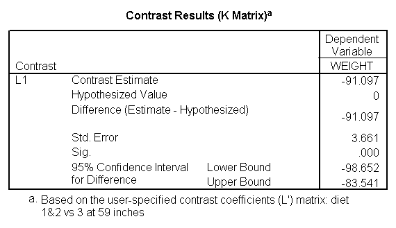
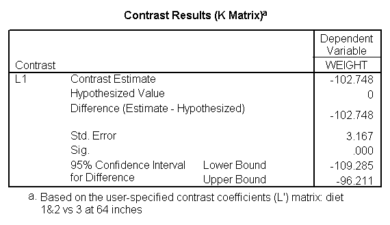
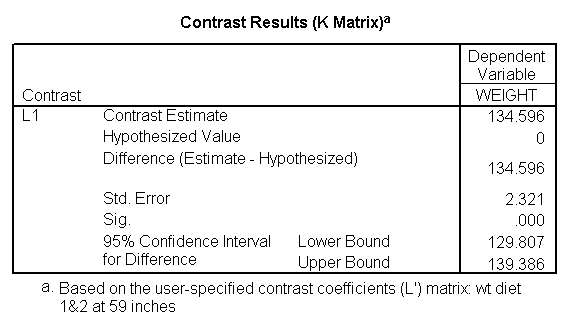
The output indicates the difference in weight between diet groups 1 and 2 combined and the control group is -91.0967 pounds at 59 inches, and this difference is significant. We could obtain that difference by taking 134.596 (the average for diet groups 1 and 2 at 59 inches) minus 225.693 (the average for diet group 3 at 59 inches). Likewise, the difference between diet groups 1 and 2 versus diet group 3 is significant at 64 inches (with a difference of -102.748 pounds) and at 68 inches (with a difference of -112.069 pounds). Despite the interaction, the control group (diet 3) always weighs more than the two diet groups combined. This is consistent with what we saw in figure 2.

6. Testing to pool slopes

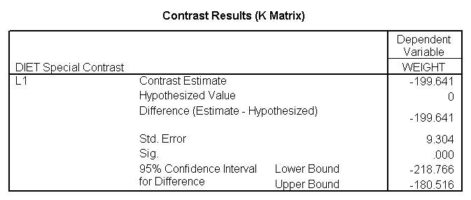
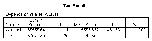
You may have noticed that the slope for diet group 1 was quite different from 2 and 3, but 2 and 3 were not so different from each other (see the graph from figure 2 and output in section 4)  Rather than estimating three separate slopes, maybe it would be better if we estimated a slope for diet group 1, and one combined slope for diet groups 2 and 3. Let's compare the slopes for diet groups 2 and 3 to see if they are different (and if they are not different they can be combined), and also test to see if the slope for diet group 1 is really different from the combined slopes for diet groups 2 and 3.

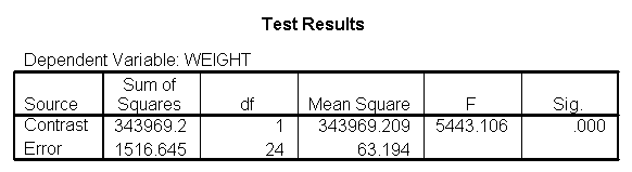
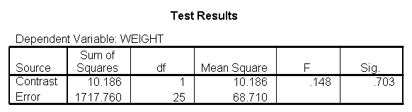
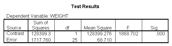
                glm weight by diet with height  /design diet height diet*height  /emmeans = tables(diet)  /print = parameter  /lmatrix "compare 1 vs 2 and 3" diet*height -2 1 1  /lmatrix "compare 2 vs 3" diet*height 0 -1 1.              

For the sake of saving space, we show just the output related to the lmatrix subcommands.

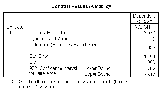
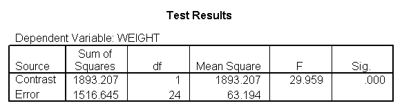
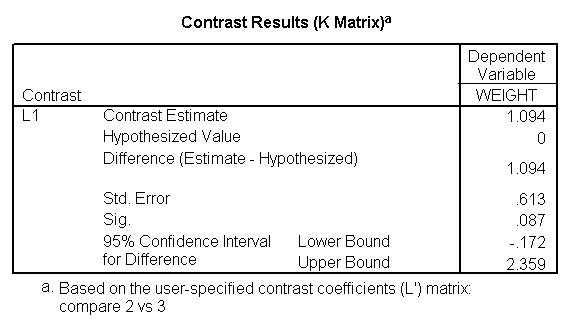
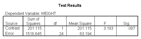
As we expected, the test comparing the slopes of diet group 1 versus 2 and 3 was significant, and the test comparing the slopes for diet groups 2 versus 3 was not significant. Because the slopes for diet groups 2 and 3 do not significantly differ, we can simplify our model by including one slope for diet group 1, and one combined slope for diet groups 2 and 3. This model has two benefits: 1) The estimate of the slope for diet groups 2 and 3 will be more stable (because it is based on more cases) than slopes computed separately. Second, as we will see later, comparisons between diet groups 2 and 3 are greatly simplified since they will have a common slope.

7. Perform tests with some pooled slopes

7.1 Overall analysis pooling slopes for diet groups 2 and 3

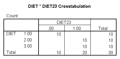
Let's see how we can can estimate a model with one slope for diet group 1, and another slope for diet groups 2 and 3. First, we will make a dummy variable that is 0 for diet group 1, and 1 for diet groups 2 and 3, called diet23.

                if diet = 1 diet23 = 0. if any(diet,2,3) diet23 = 1. execute.  crosstabs /tables = diet by diet23.              

The diet23 variable has been created successfully.

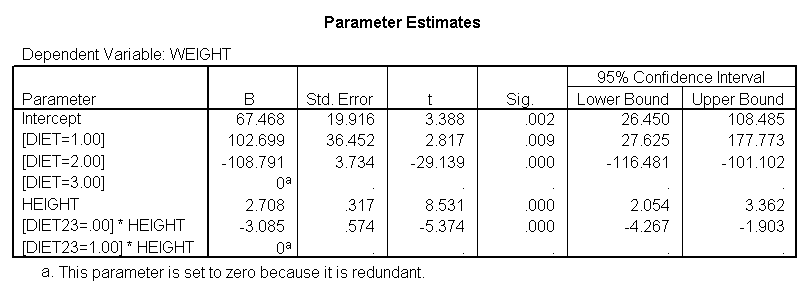
Now, we can use diet23 in our model. The variable diet is included in the /design subcommand to indicate the mean differences among the three different diet groups, and diet23*height is used to indicate that we want to estimate two slopes.

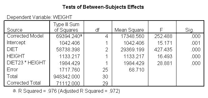
                glm weight by diet diet23 with height  /design diet height height*diet23  /print=parameter.              

Notice that diet has 2 df (since it has three levels) but the interaction of diet23*height has only 1 df (since diet23 has only two levels), whereas in section 4 the diet*height interaction had 2 df (since diet has three levels).

7.2 Comparing diet groups 1 and 2 when pooling slopes for diet groups 2 and 3

Even though we have pooled the slopes for groups 2 and 3, when we want to compare groups 1 and 2 we are comparing across groups with different slopes so we still need to use lmatrix to compare the diets at the different levels of heights and obtain the adjusted means. The first three lmatrix subcommands below compare diet groups 1 with 2 at the three levels of height (59, 64 and 68 inches). The next three lmatrix  subcommands obtain adjusted means for diet 1 at the three heights, and the next three lmatrix  subcommands obtain adjusted means for diet 2 at the three heights.

                glm weight by diet diet23 with height /design diet height diet23*height /print=parameter /lmatrix "diet 1 vs 2 at 59 inches" diet 1 -1 0 diet23*height 59 -59 /lmatrix "diet 1 vs 2 at 64 inches" diet 1 -1 0 diet23*height 64 -64 /lmatrix "diet 1 vs 2 at 68 inches" diet 1 -1 0 diet23*height 68 -68 /lmatrix "wt for diet 1 at 59 inches" intercept 1 diet 1 0 0 height 59 diet23*height 59 0 /lmatrix "wt for diet 1 at 64 inches" intercept 1 diet 1 0 0 height 64 diet23*height 64 0 /lmatrix "wt for diet 1 at 68 inches" intercept 1 diet 1 0 0 height 68 diet23*height 68 0 /lmatrix "wt for diet 2 at 59 inches" intercept 1 diet 0 1 0 height 59 diet23*height 0 59 /lmatrix "wt for diet 2 at 64 inches" intercept 1 diet 0 1 0 height 64 diet23*height 0 64 /lmatrix "wt for diet 2 at 68 inches" intercept 1 diet 0 1 0 height 68 diet23*height 0 68.              

We have omitted the portion of the output that was the same as that in section 7.1 to save space.

We can compare the results here with those of section 5.1 (which also compared groups 1 and 2, but estimated separate slopes for all three groups).  We see that the results are quite consistent, i.e., the difference between diet groups 1 and 2 are different at 59 inches, 64 inches, but not at 68 inches.

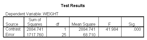
7.3 Comparing diet groups 2 and 3 when pooling slopes for diet groups 2 and 3

Because we have estimated a common slope for diet groups 2 and 3, it is easier to compare diet groups 2 and 3. Since the slopes for these two groups are parallel, we can compare these two groups at any value for height and the difference between the regression lines will remain constant. Hence, to compare diets 2 and 3, we only need diet 0 1 -1 in the lmatrix subcommand.  To obtain traditional adjusted means for each diet, you would estimate the adjusted mean at the overall mean value of height (in this case 63.13) as shown below.

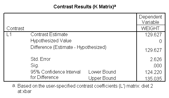
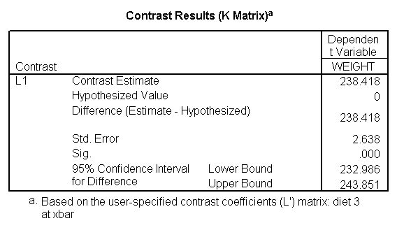
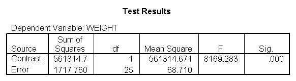
                glm weight by diet diet23 with height /design diet height diet23*height /print=parameter /lmatrix "diet 2 vs 3" diet 0 1 -1 /lmatrix "diet 2 at xbar" intercept 1 diet 0 1 0 height 63.13 diet23*height 0 63.13 /lmatrix "diet 3 at xbar" intercept 1 diet 0 0 1 height 63.13 diet23*height 0 63.13.              

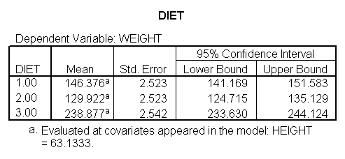
We have omitted the portion of the output that was the same as that in section 7.1 to save space.  The comparison of diets 2 and 3 is significant, and this holds true across all levels of height.  Those in diet group 2 weighed about 108.8 pounds less than those in diet group 3.  For those of average height, the adjusted mean for diet 2 was 129.6 and for diet 3 was 238.4 (and 129.6 – 238.4 = -108.8).

8. Summary

We have seen that in ANCOVA it is important to test the homogeneity of regression assumption, and if this assumption is violated we then need to estimate models that have separate slopes across groups.  This amounts to having an interaction between your covariate and your group variable, which means that when you estimate differences among the groups, you need to take the level of the covariate into consideration.  One strategy, as illustrated here, is to look at the effect of your group variable at different levels of your covariate.  In our example, when we compared the control group to diets 1 and 2, we found that the control group weighed more at three different levels of height (59 inches, 64 inches and 68 inches).  However, when we compared diets 1 and 2, we found diet 2 to be more effective at 59 and 64 inches, but there was no difference at 68 inches.  Had we not done this further investigation, we may have concluded that diet 1 was superior to diet 2 for people of all heights, not realizing that the effectiveness of the diet depended on height.

haislippanytherry40.blogspot.com

Source: https://stats.oarc.ucla.edu/spss/library/spss-libraryhow-do-i-handle-interactions-of-continuous-andcategorical-variables/